Contents:
1. Introduction
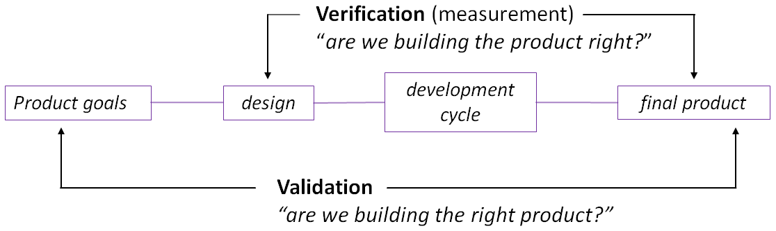
During the development and final stages of your
project you will need to verify that your product performs according to the required
specifications, for example, for accuracy, precision, efficiency, rate.
This is an
objective process where appropriate experimental data (observations) is collected and
analysed.
Figure 1: The verification and validatation cycle (simplified).
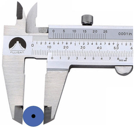
In many cases a single measurement of a parameter (e.g. the diameter of a wheel) may be sufficient given the correct used of an appropriate instrument (e.g. a Vernier caliper).
Figure 2: The diameter of a wheel is determined to be 12.1 mm to three-siginificant-figure accuracy.
More complex systems often exhibit variability due to random processes within the system (e.g. electronic noise), or within the measurement instrument/procedure (e.g. variable alignment of rulers, reading errors), or in the working environment (e.g. ambient temperature changes, random arrival of objects on a conveyor belt). In the presence of variability, we need to make repeated measurements and then apply statistical analysis, and finally interpretation of the results.
This page outlines some common basic statistical tools that you may find useful for the verification process of your product. The focus here is not only on obtaining a measurement of the performance parameter, but also an estimate of the uncertainty in the measurement. Since many other tools and procedures exist, please discuss with your supervisor which procedures and tools are appropriate for your project.
2. Sampling
If an entire population cannot be measured,
then a sub-set of the population (a sample) can provide an estimate. Consider n
repeated measurements (a sample of size n) from the population under investigation.
Each measurement is labelled vi and the collection is:
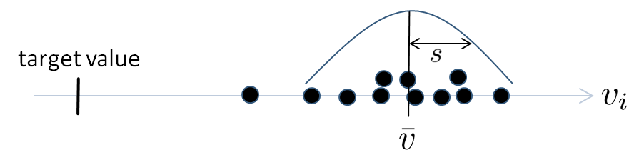
The distribution of the values may look, for example, something like below:
Figure 3: Distribution of a sample of 11 sample points.
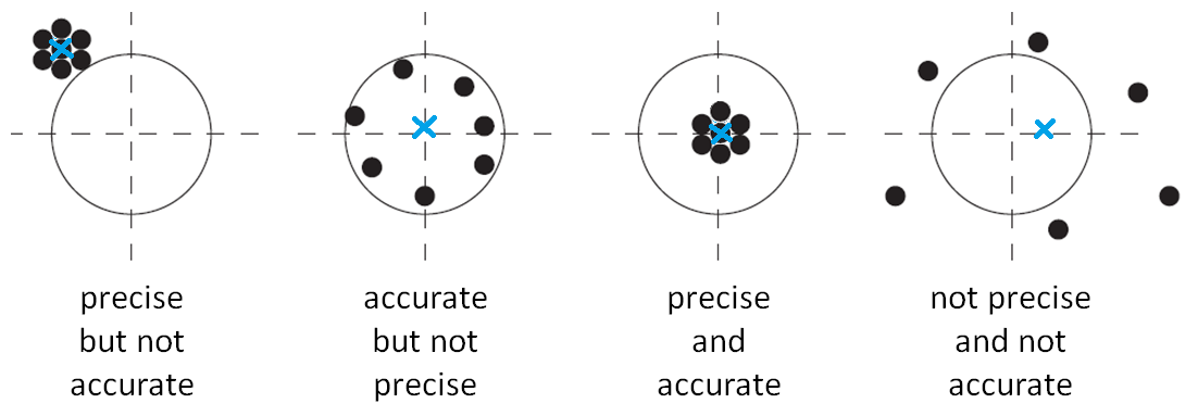
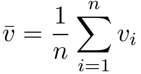
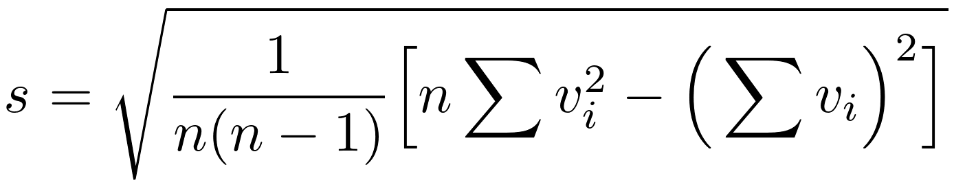
The sample mean of the values, vbar, is a estimate of the true mean (center of mass) μ of the population. The difference between μ and the design target for the population is sometimes called accuracy. The sample standard deviation, s, is an estimate of the standard deviation, σ, which is a standard measure of the variability of the process; this is sometimes called precision. These definitions of accuracy and precision are illustrated in Figure 4.
Figure 4: Illustration of accuracy and precision. Note that alternative definitions of accuracy exist; such as the maximum error in the collection, or the combined effect of the systematic and random errors.
The estimates vbar and s are calculated as follows:
For these values to be meaningful, we need an estimate of their uncertainty. This is commonly achieved by calculating a confidence interval or applying a hypothesis test. It is important to note that in both methods, uncertainty is proportional to √n; design your experiment to collect enough data for your needs.
3. Confidence intervals (ci)
A common way to express a
measured quantity and its uncertainty is to compute a confidence interval where we would
state, for example:
We are 95% confident that the parameter lies in the interval x ± Δx
or simply: x0 = x ± Δx (95% ci).
Example:
The acceleration due to gravity is determined to be g0 = 9.81 ±
0.02 m/s2 (95% ci).
This can also be written as: 9.79 <
g0 < 9.83 m/s2 (95% ci).
A 95% confidence interval means that if we were to take 100 different samples of the same sample size and compute a 95% confidence interval for each sample, then approximately 95 of the 100 confidence intervals would contain the true value of the parameter. It does not mean that there is a 95% probability that the true value is inside the current interval.
3.1 Confidence intervals for μ and σ.
In cases where the population is
approximately Normally distributed (that is symmetric
bell-shaped, with a population mean μ and population standard deviation σ), confidence
intervals for μ and σ can be computed as described below.
Confidence interval for μ
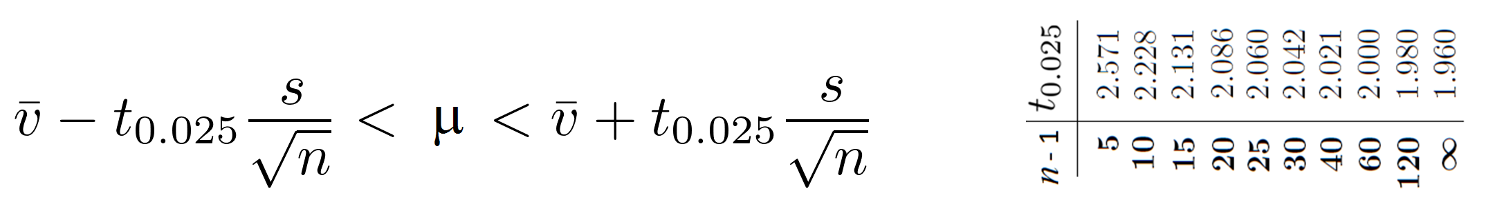
The two-sided confidence interval for μ can be
constructed as follows:
“We are 95% confident that the true mean lies in this interval.“
The value of t0.025 depends on the number of degrees of freedom,
n-1; these values are tabulated above. For other values of n-1 you can
obtain the t-value by solving the Matlab/Octave
equation:
“tcdf(t0.025,n-1)=0.975″. Alternative,
use this cdf calculator.
Confidence interval for σ
We are often interested in a single-sided
upper-bounded confidence interval for σ, for example in the case where σ is a measure of
precision:
[open the image in a new tab to get a larger version]
“We are 95% confident that the true standard deviation is less than this bound.“,
or “We are 95% confident that the precision of the process is better than this value.“.
The value of χ20.95 depends on the number of degrees of
freedom, n-1 and can be calculated by solving the Matlab/Octave
equation:
“chi2cdf(χ20.95,n-1)=0.95″.
Alternatively, use the scale formula and take the scale from the table (open the
image in a new tab to see the full size). Alternatively, use this cdf calculator.
3.2 Confidence interval for fractions (probabilities and efficiencies)
If
identical processes result in a success or fail each with a constant
success probability p then the number of successes m out of n
trials follows a Binomial
distribution.
We are often interested in measuring the success
probability p which can represent, for example, the efficiency, or
success fraction of an engineered process.
A confidence interval for p can be formed as follows:
The process is run for
n trials in which m success are observed; the point estimate for
p is then p’ = m/n. The true value of p can then expressed
as the confidence interval:
(≈ 95% ci)
This simple formulation does not work well for values of p close to 0 or 1, for such cases a proper treatment is required. The exact Clopper-Pearson interval (based on the pmf leaving an equal probability on both sides) can be constructed as follows: pLower < p < pUpper
(95% confidence interval): sum(binopdf(m:n,n,pLower)) = 0.025sum(binopdf(0:m,n,pUpper)) = 0.025
Example: n = 100 trials, m = 80 successes, and so p’ = 0.80.
  >> sum(binopdf(m:n,n,0.70816))
  ans =  0.025
  >> sum(binopdf(0:m,n,0.87334))
  ans =  0.025
and so 0.708 < p < 0.873 with 95% confidence.
The same result can be
obtained more easily from this online calculator :-).
Proof that
this actually works (reasonably) well can be seen in this c++ simulation[The simulation
suggests that the confidence level is a bit higher, more like 97%, so the c.i. is a bit
conservative. In some cases 0:m+1 works better, but my simulation might be a bit
off(?)].
Compare this to the more simple form: p = 0.80 ± 2 sqrt(0.80(1-0.8)/100) = 0.80 ± 0.08 and so 0.72 < p < 0.88 which does not allow for the asymmetry in the Binomial distribution.
3.3 Confidence interval for rates (Poisson)
We often need to measure the
rate at which a product or service can process (or create) events. This may be a simple case
of counting the number of events, n, over a period of time, t, and
expressing the rate as R = n / t. If however, the events are occuring randomly,
then there is uncertainty in this count. One class of random occurences can be modelled by
the Poisson distribution where events occur a
probability that does not change over time. Such events have a mean number of occurences per
unit time, λ.
For a Poisson process, in a time t, the measured number of events n has an
uncertainty of ≈ √n.
An approximate 95% confidence interval would be:
n0 = n ± 2√n
There are more rigorous treatments, but the above form should be a reasonable approximation as long as you record enough events, that is much more than 10. Simply increase the time period until you have collected plenty of observations of the event.
Example
n = 45 occurences are observed in a 60-second interval, and so the
observed mean rate is 45/60 = 0.75 per second.
The 95% confidence interval is therefore:
n0 = 45 ± 13.4 ⇒ 31.6 < n0 < 58.4
⇒ the mean rate λ = 45/60 ± 13.4/60
= 0.75 ± 0.22 events/second, or 0.53 < λ < 0.97 events/second (95% c.i.).
As usual with sampling, the uncertainty reduces ∝ 1/√n. For example is 450 events were observed over 600 seconds (ten times the observation period) then
n0 = 450 ± 42.4
⇒ the mean rate λ = 450/600 ± 42.4/60
= 0.75 ± 0.07 events/second, or 0.68 < λ < 0.82 events/second (95% c.i.)
Proof that n0 = n ± 2√n provides a 95% c.i. for large n can be seen in this c++ simulation.
4. Hypothesis testing
A hypothesis test provides a
method for rejecting an assumption about a population parameter based on observations (a
sample). This approach can be used, for example, to determine if a system has achieved the
required performance: if the measured performance is statistically significantly better than
the required performance then we can confidently conclude that the performance requirement
is met (and exceeded [design your product to be better than the requirements]).
The following sections present examples of testing a hypothese for μ, σ, p amd λ.
4.1 Hypothesis test for μ and σ.
Below are examples of hypothesis tests
performed for a population that is approximately Normally distributed (that is symmetric
bell-shaped, with a population mean μ and population standard deviation σ) and a sample of
size n results in observations of the sample mean vbarobs and
sample standard deviation sobs.
Hypothesis test for μ
Consider a process that is required to have an
accuracy, μ, better than (less than) a value μ0. One strategy would be to design
the process to a higher accuracy and make an observation of vbar that is
statistically significantly less than μ0 to rule out the chance of a statistical
fluctuation.
In a hypothesis test, we can reject the hypothesis μ = μ0 in
favor of μ < μ0 if the following computed probability (P-value) is
“small”:
This can be solved using Matlab/Octave, or by using this cdf calculator.
Here,
“small” would be a few percent or less for a significant result, and 1% or less
for a very significant result (smaller is better). If the probability is large then the
hypothesis cannot be rejected and we are not confident that that the accuracy requirement
has been met.
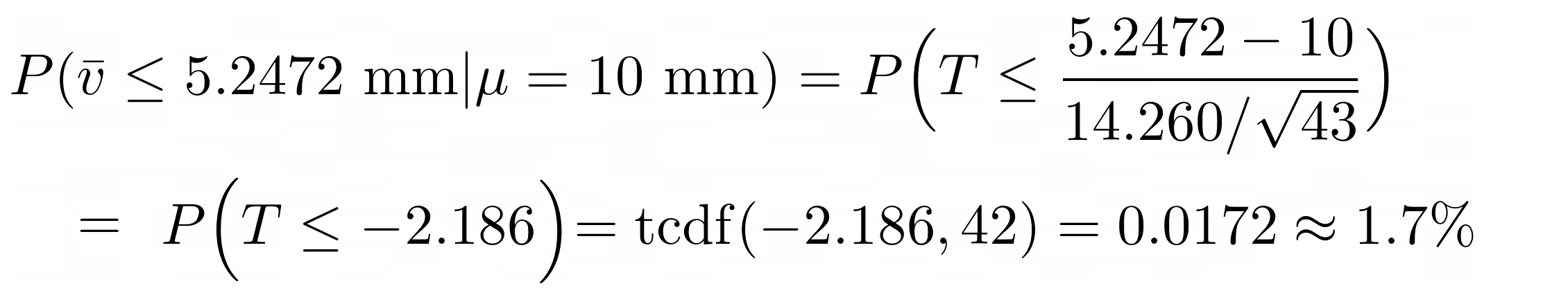
Example
43 observations are made for placements by a pick-and-place robot; the sample mean
placement is calcuated to be 5.2472 mm from the target with sample standard deviation of
14.260 mm. The robot is required to have an accuracy (μ) of better than 10 mm. The sample
mean is well within the requirement, but this could be a statistical fluctuation. The
hypothesis test for μ is as follows.
The probability that we would observe a sample mean of 5.2473 mm when the true mean is 10 mm, is just 1.7%. This is a significant (small) P-value and so we can reject the hypothesis μ = 10 mm in favor of μ < 10 mm and so we conclude that accuracy requirement is satisfied.
Hypothesis test for σ
Consider a process that is required to have a
precision, σ, better than (less than) a value σ0. One strategy would be to design
the process to a higher precision and make an observation of s that is
statistically significantly less than σ to rule out the chance of a statistical
fluctuation.
In a hypothesis test, we can reject the hypothesis σ = σ0 in
favor of σ < σ0 if the following computed probability (P-value) is
“small”:
This can be solved using Matlab/Octave, or by using this cdf calculator.
Here,
“small” would be a few percent or less for a significant result, and 1% or less
for a very significant result (smaller is better). If the probability is large then the
hypothesis cannot be rejected and we are not confident that that the precision requirement
has been met.
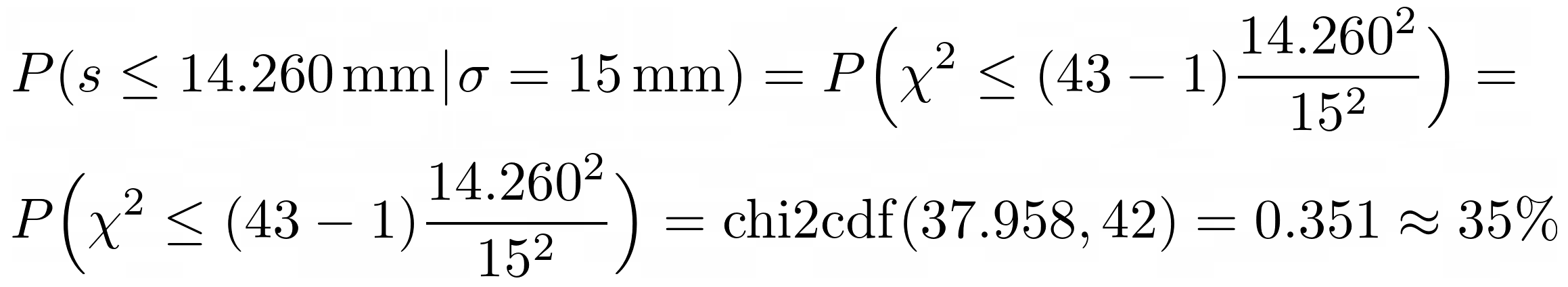
Example
43 observations are made for placements by a pick-and-place robot; the sample mean
placement is calcuated to be 5.2472 mm from the target with sample standard deviation of
14.260 mm. The robot is required to have a precision (σ) of better (smaller) than 15 mm. The
sample standard deviation is smaller, but this could be a statistical fluctuation. The
hypothesis test for σ is as follows.
Since we have a high probability (35%) that we would observe a sample standard deviation of 14.260 mm (or less), given a true standard deviation of 15 mm, then we cannot reject the hypothesis σ = 15 mm in favor of σ < 15 mm. We cannot say that the precision requirement is satisfied. In this case we would increase the sample size and/or improve the robot precision.
4.2 Hypothesis test for fractions (probabilities and efficiencies)
If
identical processes result in a success or fail each with a constant
success probability p then the number of successes m out of n
trials follows a Binomial distribution. We
are often interested in designing a system with high efficiency, or success
fraction for the process being performed; that is p is large. If a system
is required to have a p value of at least p0 then one strategy
would be to design the process to have a larger value of p with the hope of
observing a value p’ = m/n that is statistically significantly greater than
p0 to rule out the chance of a statistical fluctuation.
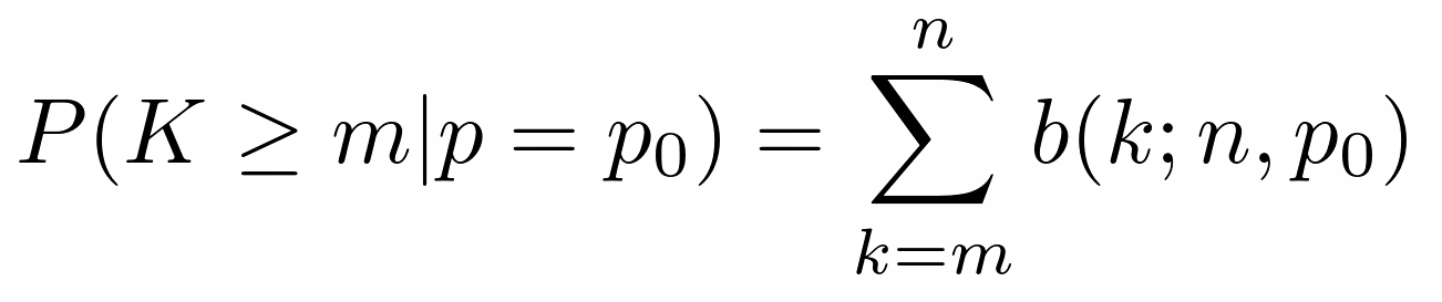
In a
hypothesis test, we can reject the hypothesis p = p0 in favor of p
> p0 if the following computed probability (P-value) is
“small”:
where m is the observed number of sucessess out of n trials.
This can be
computed with Matlab/Octave as follows:
sum(binopdf(m:n,n,p0))
Here, “small” would be a few percent or less for a significant result, and 1% or less for a very significant result (smaller is better). If the probability is large then the hypothesis cannot be rejected and we are not confident that that the requirement for p has been met.
Example
A pick-and-place robot is required to pick up without dropping at least 70%
(p=0.7) of items on a conveyor belt. During a test, the robot is observed to pick up without
dropping 80 out of 100 items (the observed value is p’ = 0.8). The hypothesis
test for p is as follows:
You can also obtain this P-value here.
The P-value is small (significant), so we can reject the hypothesis that p = 0.7 in
favor of p > 0.7 and so the requirement is met.
Remember that the 95%
confidence interval was 0.708 < p < 0.873 which also excludes p =
0.7.
4.3 Hypothesis test for rates (Poisson)
See the introduction to the
Poisson process given in Section 3.3.
For a Poisson process, in a time t, the measured number of events m has an
uncertainty of ≈ √m.
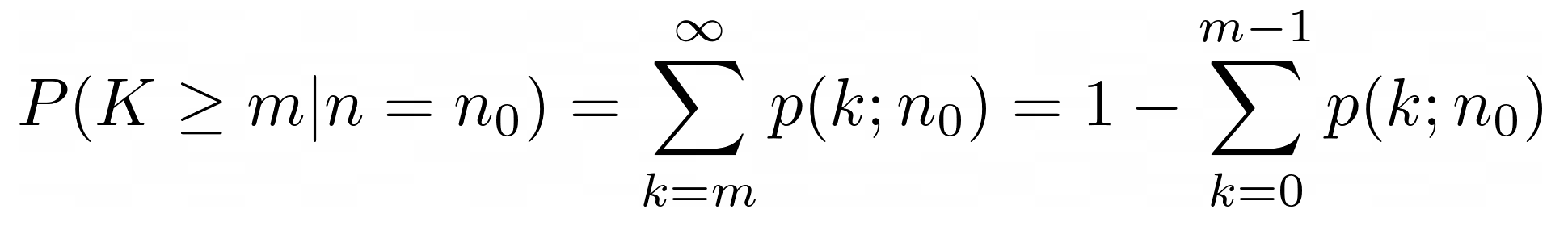
If the mean number of events, for this time interval, is required to
be n0, then a hypothesis n = n0 can be rejected in favor of
n > n0 if the following computed probability (P-value) is
“small”:
Here, “small” would be a few percent or less for a significant result, and 1% or less for a very significant result (smaller is better). If the probability is large then the hypothesis cannot be rejected and we are not confident that that the requirement has been met.
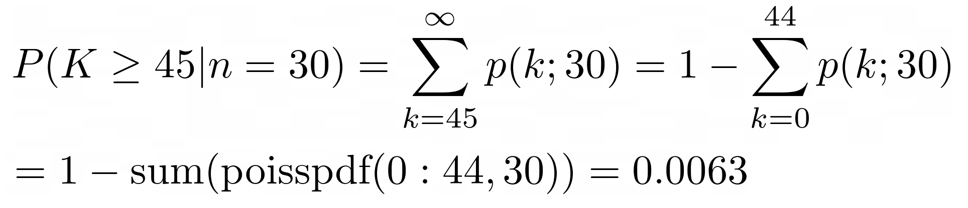
Example:
m = 45 events are observed in a 60-second interval, and so the observed
mean rate is 45/60 = 0.75 per second.
The required rate is 0.5 per second ⇒ n =
0.5 x 60 = 30 events. In a the following hypotheisis test, we attempt to reject n =
30 in favor of n > 30.
(see also this online calculator)
The P-value is very signficant (very small), less than 1%, and so reject the hypothesis and
can conclude that the requirement for the mean rate, λ > 0.5, is satsisfied.
This is
consistent with the above confidence interval result of 0.53 < λ < 0.97 events/second
(95% c.i.) which excludes λ = 0.5.
Comments/corrections to Dr. Tarkan AYDIN (tarkan.aydin@bau.edu.tr)